How To Total A Row In Google Sheets
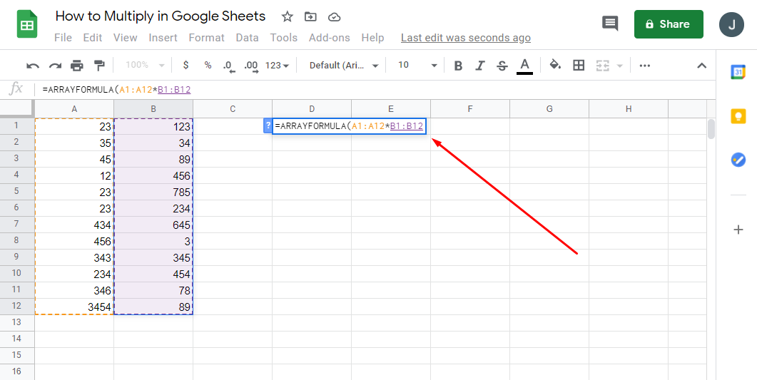
QUERY ArrayFormula if len A2A A2A TotalB2DSelect Col1sum Col2 Sum Col4 where Col1 is not null group by Col1 label sum Col2Sum Col4 As you can see it returns the subtotal rows to. Highlight the cells you want to calculate.
How To Group Rows And Columns In Google Sheets
One is normal filtering the data and the second one is adding a total row to the end.
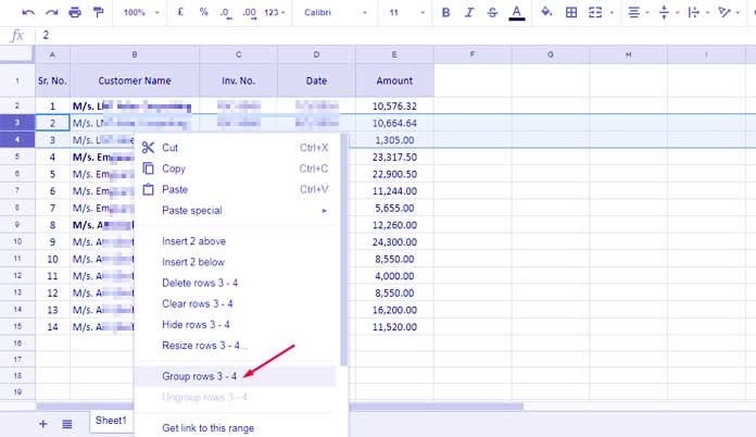
How to total a row in google sheets. ROWcell_reference cell_reference is the address reference to the cell whose row. Select the entire row A2 and right click and select Group row. Replace each of the SUM formulas with formulas using the SUBTOTAL function eg.
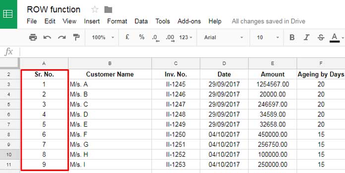
The ROW formula is one of the lookup functions available within Google Sheets. To use a formula to subtract two cell values in Google Sheets follow these steps. Query A1H12Select where DSafety Helmet The above Google Sheets QUERY formula filters column D.
Next highlight the total row. Whereas in Google sheet we have to. This SUMIFS formula requires a manual action to populate the result in the rows below.
There are two steps involved. This opens the function menu. Next to Explore youll see Sum.
Then select the rows 4 to 11 and similarly apply the grouping. On your computer open a spreadsheet in Google Sheets. Click the file you want to edit.
Click the cell where you want to place the result. How to Count Rows Between Two Values in Google Sheets Click on any cell to make it the active cell. We will discuss using the sign and also using the SUM function.
You can quickly calculate the sum average and count in Google Sheets. This feature doesnt work for some numbers or currency formats. Add A Pie Chart Office Support.
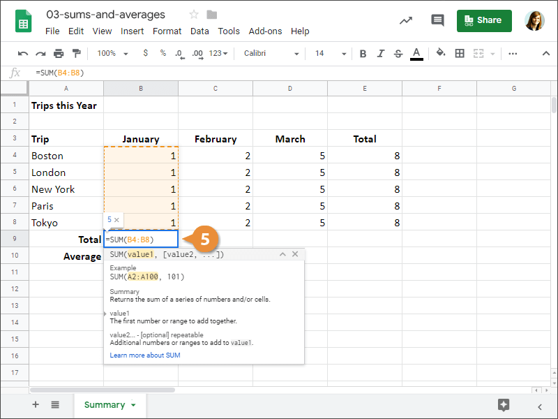
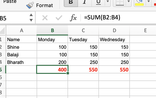
Both work but th. Highlight the cell and set up the sum range for the number of rows you are totalling. INDEXSheet1to get the value from the column with the total amount for example.
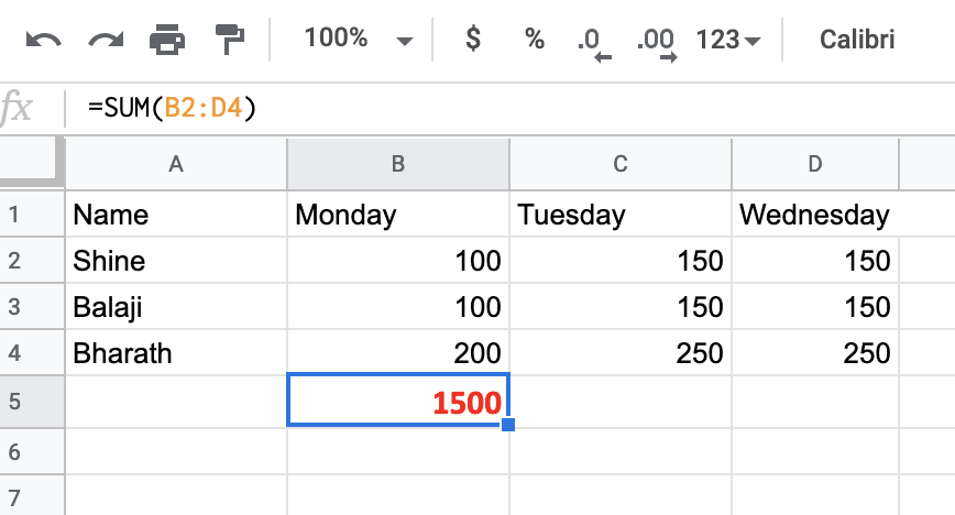
If you are not familiar with the basics of spreadsheet formulas check out my Spreadsh. Select the cell where you want the result to appear cell C2 Put an equal to sign in the cell to start the formula. Learn the different ways to total columns of numbers in your spreadsheet.
How To Hide Grand Total Row In Google Sheets Pivot Charts Josh Gler. However by using the SUBTOTAL Function in Google Sheets you can solve this problem. For this guide I will be selecting E3 where I want to show my result.
It should say Sheet1 with the being the row number for the total. If you look up at the formula bar you will notice an equal to sign appearing there too. SUBTOTAL 9C2C5 When you calculate the grand total again using the SUBTOTAL function it wont double count the values.
Create Outstanding Pie Charts In Excel Pryor Learning Solutions. INDEXDataH4HMATCHTotalDataA4A01 which assumes the label Total is in Data. Its near the top-right corner of the sheet.
You can use the same SUMIFS formula to return the last 7 30 and 60 days total from today in Google Sheets. In this video I demonstrate how to sum a column or row of sales data. We will combine F1 and F8 formulas in the final step.
This can be any blank cell on the sheet. Next type the equal sign to begin the function and then followed by the name of the function which is our match or MATCH not case sensitive. Total To see more calculations click Sum.
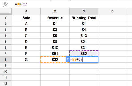
RIght click and choose protect range. If for some reason you want to do running total ROW-wise this is the formula that works for me when you have a POSITIVE range of values starting from D1 all the way up to columns running over row 1 ArrayFormulaifD11transposeMMULTtransposetransposeCOLUMND11. Column A and the actual total amount in Data.
MATCHTotalSheet0 to find what row the Total label is in then. Its at the top of the menu. In the bottom right find Explore.
Follow this grouping for all the groups. 2 Recommended Answers In Excel to get sum of different rows select complete rows and columns and click AutoSum will get total sum for each rows. Steps Download Article.
A sidebar will open with a field for the protected range. That means you should drag the fill handle in cell A2 down. Pie Chart Color Scale Tibco Munity.
It gives us the row number where the specified cell or a range of cells are located. I mean for the rows 13 to 18 20 to 21 and 23 to 25.

Google Sheets Group Rows And Columns Youtube
How To Multiply In Google Sheets Using Numbers Cells Or Columns
Sums And Averages Customguide

How To Hide A Row In Google Sheets Solve Your Tech
Autosum In Excel And Sum In Google Sheet Google Docs Editors Community
Autosum In Excel And Sum In Google Sheet Google Docs Editors Community
Running Total Calculations In Google Sheets Using Array Formulas

How To Sum A Column In Google Sheets Easy Formula Spreadsheet Point

How To Total A Column In Google Sheets Using Sum Function All Things How
Auto Serial Numbering In Google Sheets With Row Function
How To Add Up A Column In Google Spreadsheet Youtube
![]()
Insert Blank Rows Using A Formula In Google Sheets
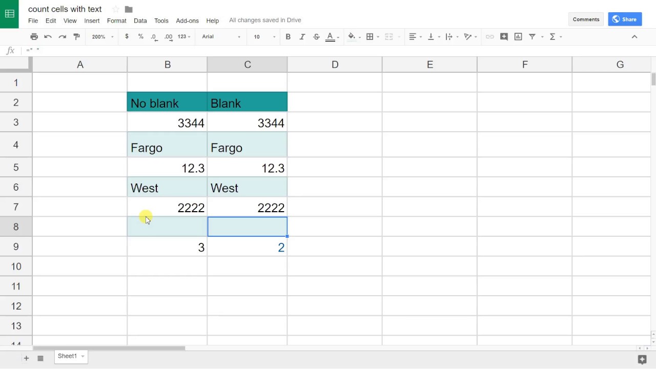
Google Sheets Count Cells With Text Only Not Numbers Youtube
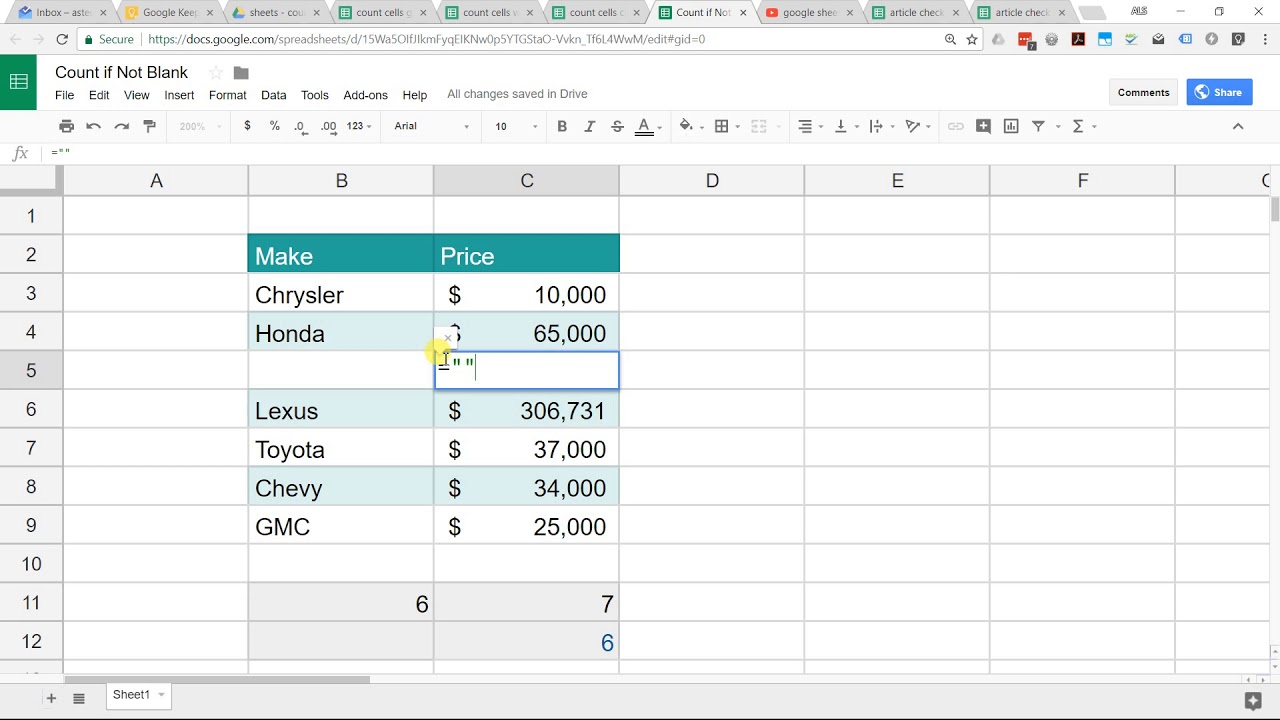
Google Sheets Count Cells That Are Not Blank Youtube

How To Sum A Column In Google Sheets Mobile Apps Desktop

Google Sheets Group Rows And Columns With Linked Example File

How To Group Rows Columns In Google Sheets Step By Step Spreadsheet Point

Google Sheets Group Rows And Columns With Linked Example File
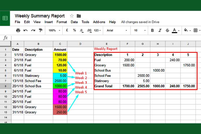
How To Create A Weekly Summary Report In Google Sheets