How To Calculate Filter Sum In Excel
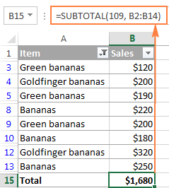
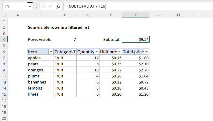
It looks like this. Enter the Subtotal formula to sum the filtered data.
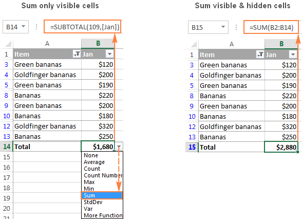
Excel Sum Formula To Total A Column Rows Or Only Visible Cells
This is where you will use the Subtotal formula.
How to calculate filter sum in excel. Change the letters and numbers in parenthesis to fit your workbook. Right-click Hide use this version instead. When you filter data getting the SUM of only the visible part of the data can be a challenge.
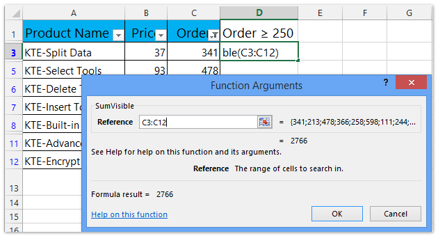
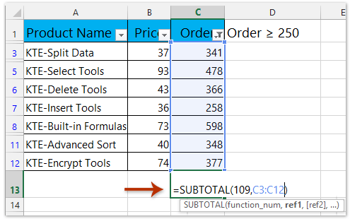
Will run until find a blank cell While RangeA iValue this check if actual value of column A is equal to before value of column A if true just add the column. SUBTOTAL9 F5F14 which returns the sum 954 the total for the 7 rows that are still visible. Save this code and enter the formula SumVisible C2C12 into a blank.
How to Calculate the Sum of Cells in Excel. A SUBTOTAL formula will be inserted summing only the visible cells in. You can see there is no change in the totals.
While filtering you must keep in mind that checkbox nex to the required name is only checked. SUMPRODUCTSUBTOTAL3OFFSETB6B19ROWB6B19-MINROWB6B191 B6B19NellyC6C19 B6B19 contains the criteria that you want to use the text Nelly is the criteria and C6C19 is the cell values you want to sum and then press Enter key to return the result as. Reading a SUBTOTAL formula.
SUBTOTAL109 F5F14 Using 109 for the function number tells. Click below the data to sum. Because the list is filtered a SUBTOTAL formula is inserted instead of a SUM formula.
Learn how to SUM only filtered data in Excel. Click anywhere in the data set. The first method is to temporarily view the subtotal for selected cells in the status bar at the bottom of the Excel window.
This is because we have used the SUM Function. You can use the AutoSum icon after applying a filter. Sub SUM Dim i j k As Integer i 2 j 2 RangeD1Value NAME RangeE1Value VALUE copy the first value of column A to column D RangeD2Value RangeA2Value cycle to read all values of column B and sum it to column E.
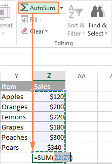
The Subtotal formula is. After that select the cell immediately below the column you want to total and click the AutoSum button on the ribbon. Once you click Excel will automatically add the sum to the bottom of this list.
Once you click Excel will automatically add the sum to the bottom of this listAlternatively you can type the formula SUM D1D7 in the formula bar and then press Enter on the keyboard or click the checkmark in the formula bar to execute the formula. Alternatively you can type the formula SUM D1D7 in the formula bar and then press Enter on the keyboard or click the checkmark in the formula bar to execute the formula. Apply filter on data.
Filter drop downs display in column headings. To do this youll select the cells you want to find the total for and the total for those cells appears in the AutoCalculate pane on the right side of the status bar. There are two ways you can find the total of a group of filtered cells.
If you use SUM function for it it will show you the SUM of th. Click Insert Module and paste the following code in the Module window. Sumrange This is the standard way to find a total.
1 2 3 4 5 6 7 8 9 10 11 Function SumVisible. The subtotal function can if we ask it nicely ignore any values hidden by the autofilter. Change the letters and numbers in parenthesis to fit your workbook.
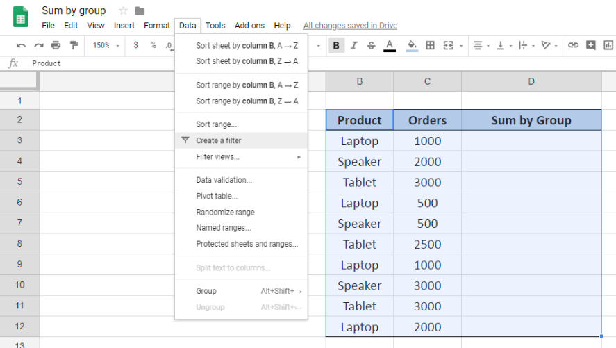
But as you can see once you use this formula and change the anything from the filtered drop-down menu the sales total doesnt change with it. Hold down the ALT F11 keys and it opens the Microsoft Visual Basic for Applications window. Click the Sort Filter drop down from the Editing group.
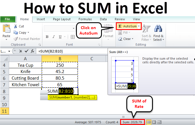
So how do you get the total to change with changes you make on the filter. On Excels Standard toolbar click the AutoSum button or on the keyboard press the Alt key and tap the equal sign key Alt. If you are hiding rows manually ie.
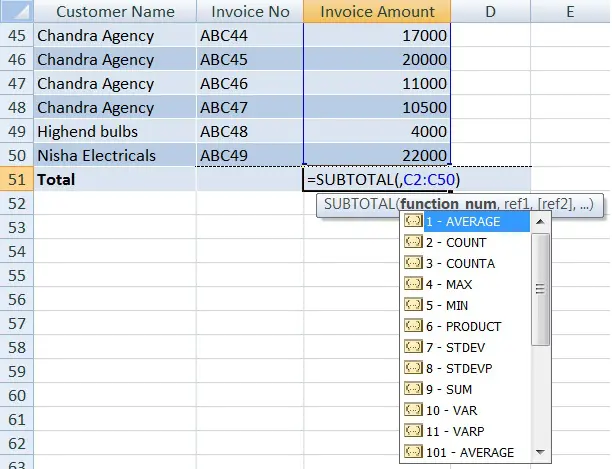
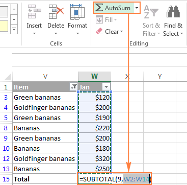
The function_num argument tells the subtotal function what sort of calculation you want it to do. Simply click AutoSum-- Excel will automatically enter a SUBTOTAL function instead of a SUM function. SUBTOTAL function_numref1 ref2.
Just organize your data in table Ctrl T or filter the data the way you want by clicking the Filter button. This tutorial will cover two quick and easy ways to ensure you get the SUM of only filtered data in ExcelTimes. Normally the AutoSum icon inserts a SUM function.
Click Home from the Ribbon. The formula used is. This function references the entire list D6D82 but it evaluates only the filtered.
When you apply a filter and then use AutoSum Excel will insert a SUBTOTAL function instead. To sum the filtered values in column C based on the criteria please enter this formula. SUM C2C50 Lets filter the table for a particular customer say Abhishek Cables.
This function will ignore rows hidden by the Filter command. Select the cell where you want the grand total.

How To Use The Excel Sum Function Exceljet
Using The Subtotal Function To Sum Filtered Data In Excel Microknowledge Inc

How To Sum Only Filtered Or Visible Cells In Excel
How To Sum In Excel Examples On Sum Function And Autosum In Excel
Excel Formula Sum Visible Rows In A Filtered List Exceljet
How To Sum Filtered Data Using Subtotal Function In Excel Exceldatapro
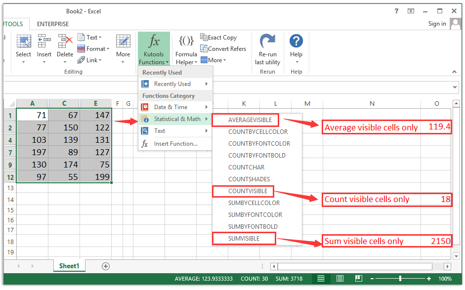
How To Sum Only Filtered Or Visible Cells In Excel
Excel Sum Formula To Total A Column Rows Or Only Visible Cells

How To Sum Only Filtered Or Visible Cells In Excel

How To Count Sum Cells Based On Filter With Criteria In Excel

How To Sum Only Filtered Or Visible Cells In Excel
Excel Formula Sum By Group
Excel Sum Formula To Total A Column Rows Or Only Visible Cells
How To Sum Only Filtered Or Visible Cells In Excel

How To Count Sum Cells Based On Filter With Criteria In Excel
Excel Sum Formula To Total A Column Rows Or Only Visible Cells
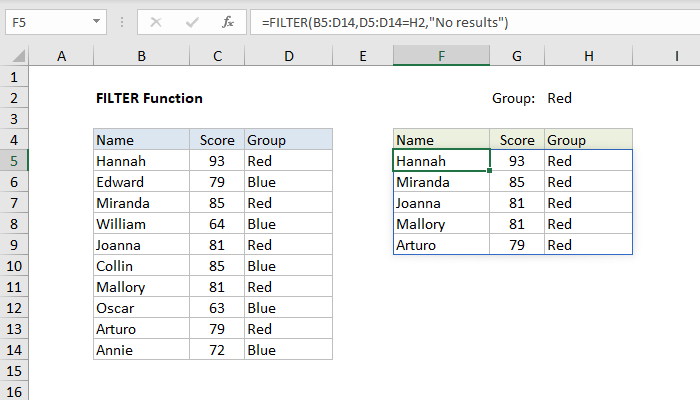
How To Use The Excel Filter Function Exceljet
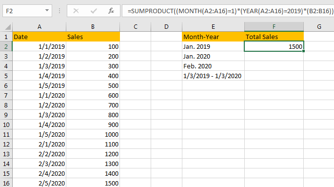
How To Sum Values Based On Month And Year In Excel Free Excel Tutorial
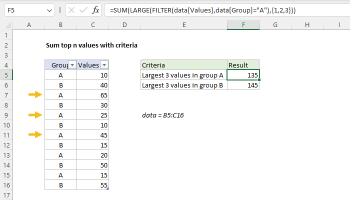
Excel Formula Sum Top N Values With Criteria Exceljet