How To Add Multiple Columns In Excel Graph
How To Add Minor Gridlines In An Excel Chart. Click the chart and study the highlighted areas in the source data.

Multiple Bar Graphs In Excel Youtube
Choose the stacked column stack option to create stacked column charts.
How to add multiple columns in excel graph. By following this method you can addshow task names next to the Gantt Chart bars in Excel 365. 7 s to make a professional looking line graph in excel or powerpoint think outside the slide how to add total labels stacked column chart in excel how to make a line graph in excel 3 ways to make lovely. XY scatter or bubble chart.
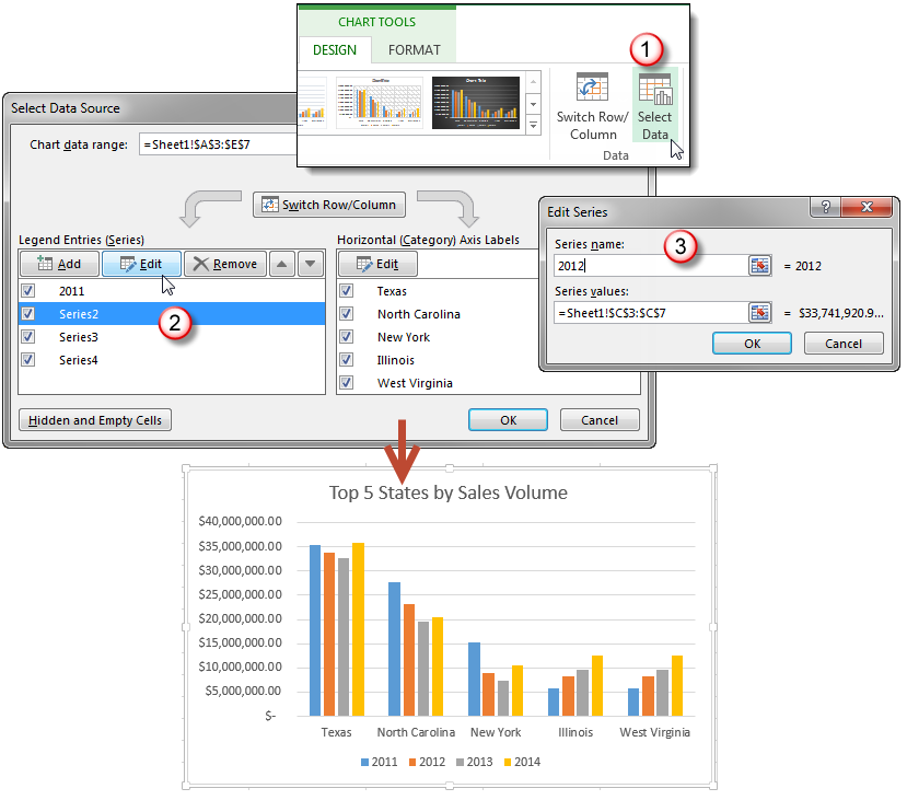
Assume your data is in the range A1F18 with W in columns AC and D in columns DF. Click on the chart youve just created to activate the Chart Tools tabs on the Excel ribbon go to the Design tab and click the Select Data button. Right-click the chart and then choose Select Data.
How to Quickly Create a Gantt Chart in Excel 365 Step by Step. Now click on Insert Tab from the top of the Excel window and then select Insert Line or Area Chart. In the chart source dialog change the chart data range to include the desired data.
Add One Trendline For Multiple Peltier Tech. Click on Insert and then click on column chart options as shown below. On the Series tab click Add.
Create a stacked clustered column chart in Excel. In one or multiple columns or rows of data and one column or row of labels. The Select Data Source dialog box appears on the worksheet that contains the source data for the chart.
Select combo from the All Charts tab. You can see the below chart. Highlight Rows Between Two Strings in Excel 365 Formula Rules.
In columns placing your x values in the first column and your y values in the next column. Also we can use a shortcut key altF11. For bubble charts add a third column to specify the size of the bubbles it shows to represent the data points in the data series.
Leaving the dialog box open click in the worksheet and then click and drag to select all the data you want to use for the chart. After insertion select the rows and columns by dragging the cursor. After selecting the data as mentioned above and selecting a stacked column chart.
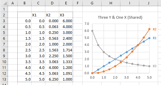
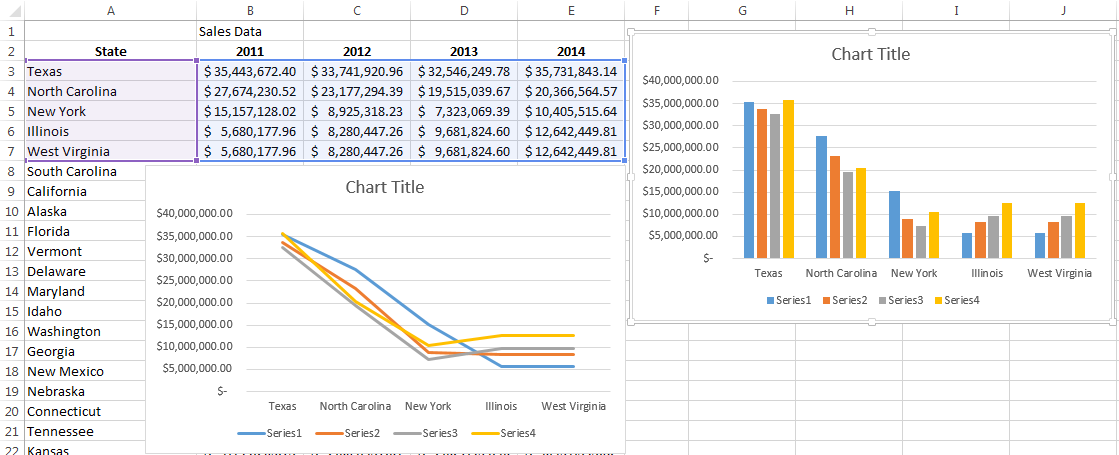
Highlight Distinct Values in Excel 365. From the above chart we can observe that the second data line is almost invisible because of scaling. Click and drag the corner of the blue area to include the new data.
Click on Insert Ribbon Click on Column chart More column chart. To create a combo chart select the data you want displayed then click the dialog launcher in the corner of the Charts group on the Insert tab to open the Insert Chart dialog box. Or click the Chart Filters button on the right of the graph and then click the Select Data link at the bottom.
In the chart source dialog click the Add button and specify the location of the new series. Right click the Chart and choose Source Data. In this video I show you how to copy the same chart multiple times and then change the cell references it is linked to in order to make lots of similar chart.
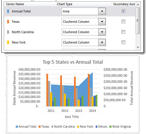
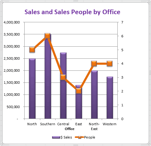
Then in Format Data Series dialog check Secondary Axis in the Plot Series On section and click the Close button. Select For A Chart Excel. In Column chart options you will see several options.
From the pop-down menu select the first 2-D Line. How to Highlight the XLOOKUP Result Cell in Excel. If we want to change anything so excel allows us.
Click the Chart icon choose XY Scatter and the Chart type you want and click Finish. Right click a column in the chart and select Format Data Series in the context menu. Select the data range and insert a chart first by clicking Insert and selecting a chart you need in the Chart group.
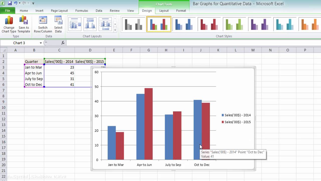
Choose the clustered column chart Click on Ok. After arranging the data select the data range that you want to create a chart based on and then click Insert Insert Column or Bar Chart. Select the range A1A18 together with range D1D18 hold down Ctrl to make the second selection.
This visualization is default by excel. Multiple Value A Amcharts. Select the chart type you.
Right click the data series bar and then choose Format Data Series see screenshot.
Multiple Series In One Excel Chart Peltier Tech
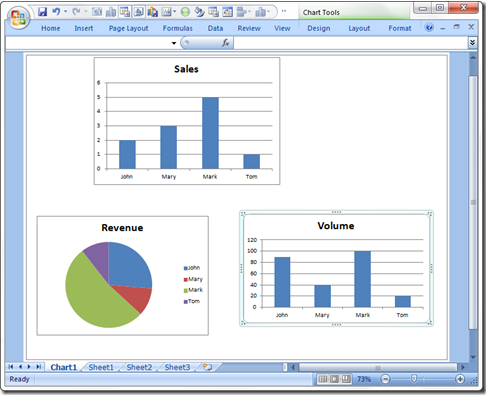
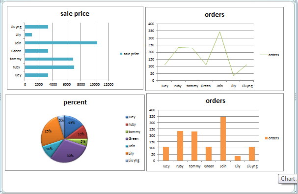
How To Add Multiple Charts To An Excel Chart Sheet Excel Dashboard Templates
How To Quickly Make Multiple Charts In Excel Youtube

How To Create Multi Category Chart In Excel Excel Board
Working With Multiple Data Series In Excel Pryor Learning Solutions
How To Color Chart Based On Cell Color In Excel
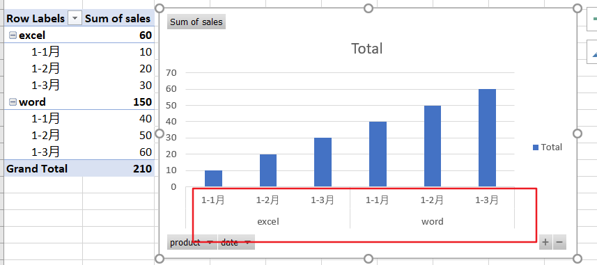
How To Create A Chart With Two Level Axis Labels In Excel Free Excel Tutorial
Working With Multiple Data Series In Excel Pryor Learning Solutions
Working With Multiple Data Series In Excel Pryor Learning Solutions

Plot Multiple Lines In Excel Youtube
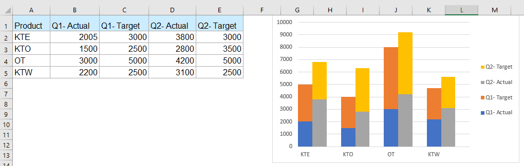
How To Create A Stacked Clustered Column Bar Chart In Excel
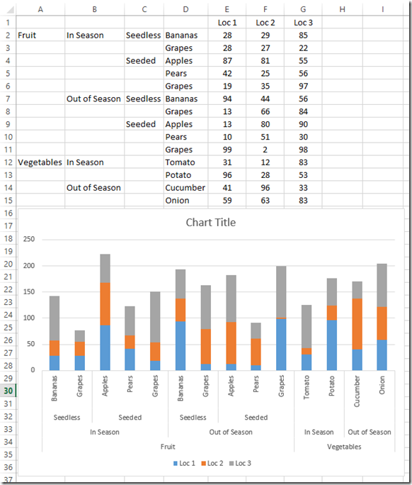
How To Graph Three Sets Of Data Criteria In An Excel Clustered Column Chart Excel Dashboard Templates
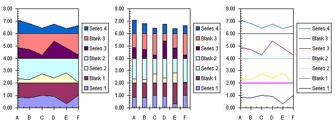
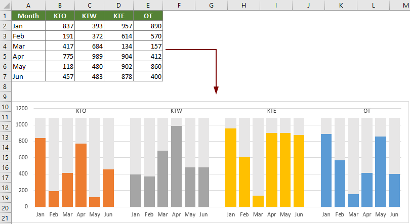
Stacked Charts With Vertical Separation
Simple Bar Graph And Multiple Bar Graph Using Ms Excel For Quantitative Data Youtube
Create Multiple Series Histogram Chart Quickly In Excel
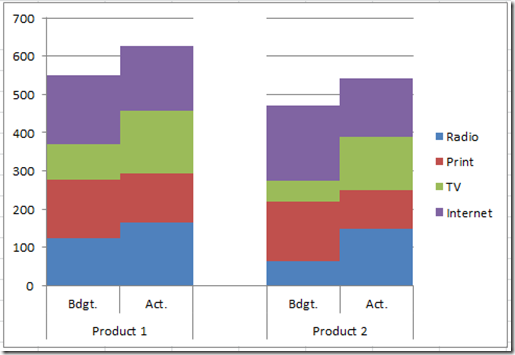
How To Easily Create A Stacked Clustered Column Chart In Excel Excel Dashboard Templates
Tips Tricks For Better Looking Charts In Excel
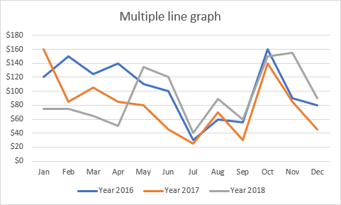
How To Make A Line Graph In Excel
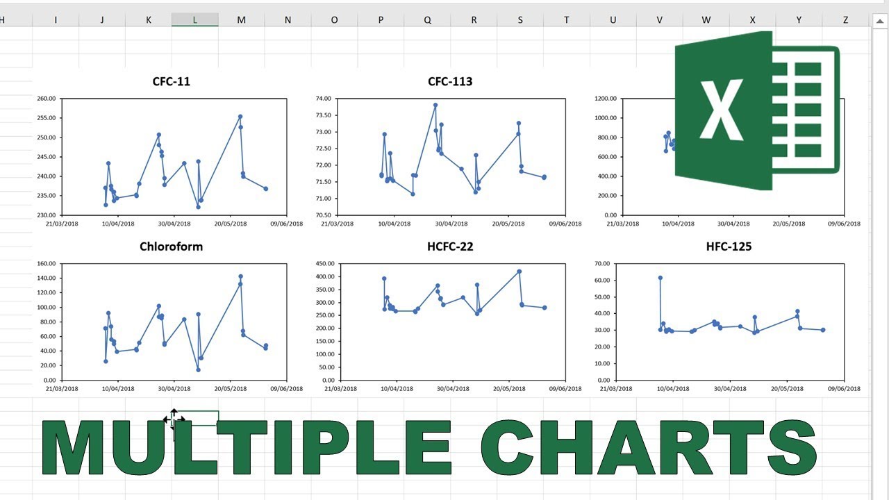
How To Display Multiple Charts In One Chart Sheet